Estimating the quality of the final fit -- an investigation
 Can we estimate the quality of the landmark positions
generated by the Active State Model?
Using the simple technique tried here, the answer is no.
Can we estimate the quality of the landmark positions
generated by the Active State Model?
Using the simple technique tried here, the answer is no.
We measure the quality of fit as the mean pixel distance
of the automatically located landmarks.
The pixel distance of a landmark
is defined to be the distance in pixels of the landmark from its correct position
(taking the "correct position" as the manually landmarked position).
Our task is devise a scheme to estimate this mean pixel distance on images
where the manual landmarks are not available.
The approach used in this investigation estimates the pixel
distance of the automatically located landmarks by linear regression
on the profile distances of those landmarks.
(The profile distance is defined as the Mahalanobis distance of
the profile from the mean profile for that landmark, equation 2.6 in the
masters thesis.)
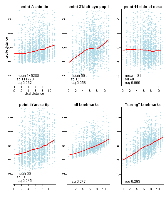
The graphs on this page plot the normalized profile distance
against the pixel distance for a landmark or a combination of landmarks.
The graphs show that
the variance of profile distances is too high
to use them to estimate pixel distances.
Details
The graphs were created by repeating the following
steps for each image in the XM2VTS set (2360 images):
- Displace the manually landmarked shape by
a random x and a random y distance.
These distances are integers drawn uniformly from -8 to +8 inclusive.
The pixel distance is the root of the sum of the squared x and y distances.
- Measure the profile distance at each landmark.
- Scale each profile distance by subtracting the mean and
dividing by the standard deviation of the profile distance.
Scaling allows us to sum the profile distances for the final two graphs.
The mean and standard deviation for each landmark are calculated over
all 2360 images, and are printed for reference at the bottom of each graph.
These are much larger for 1D profiles (such as the chin tip) than for
2D profiles (such as the eye pupil), but that is an implementation detail.
Note that profile distance for point 44 (on the side of nose) in uninformative.
This indicates that this and similar points should possibly not be included
in the Active Shape Model (although the current version of Stasm does use them).
- Plot the scaled profile distance as one blue dot in the graph for that landmark.
The distance is measured for all landmarks, but
only a few representative landmarks are graphed here.
The red line is a lowess fit to the points. (If you don't know what
a lowess
fit is, think of it as a glorified moving average.)
The rsq figure displayed at the bottom of each graph
is the R-Squared for a linear model fitted to the points
i.e. it is the fraction of variance explained by a least squares linear fit.
The non-linearity of the lowess lines indicate that fitting a linear model
is only more-or-less justified,
but the linear model does allow us to quantize the spread of the profile distances.
The all landmarks graph was created by summing the distances
for all 68 XM2VTS landmarks.
We see an R-Squared of 0.247, higher than the value
for the individual points but still not enough to be usable.
And this R-Squared is higher than it would be for real data, because (i) in
our simulated data all landmarks are displaced by the same amount for each image,
so there is a high (in fact, perfect) correlation between the pixel distances
for the different landmarks,
and (ii) we are testing on the training set, not on independent data.
The strong landmarks graph is
in an effort to improve the R-Squared over the all landmarks graph
by using only "strong" landmarks
--- but the new R-Squared of 0.293 is still not good enough to be useful.
The strong landmarks were chosen somewhat arbitrarily to be
27, 28, 30, 31, 32, 33, 35, 36, 41, 46, 47.
Landmarks are numbered using the XM2VTS scheme as shown in this
figure,
reproduced from Appendix A of the master's thesis.
Ranking the fits
In spite of the above results,
given an ASM fit it may be that the rank of the pixel distances
across landmarks can be approximated by the rank of the profile distances.
Then you would be able to determine if the left eye is
better than the right eye, for example.
Whether this would work (we haven't tried it) could be established
by using a measure such as Spearman's rank correlation
on the test data.
Another technique
The amount a point is moved to conform to the shape model can
be used as a rough indication of fit.
This technique could perhaps be combined
with the technique presented in the first section above.
A similar idea to weight the points can be found in
section 5.2 of Cootes et al.
"Building and Using Flexible Models Incorporating Grey-Level Information".
Oct 2008
Back to Stasm homepage